By Jillian Byrnes, Monique Dacanay, Kaycee DeArmey,  Alana Drumgold, Ariyana Smith*, and Wisdom Talley*.

*Ariyana and Wisdom helped the group work through the problem set but were unfortunately unable to attend camp during the blog writing.

A mathematical knot is a loop in three-dimensional space that doesn’t intersect itself, and knot theory is the topological study of these knots. Two knots are considered to be equivalent if they can be stretched or bent into each other without cutting or passing  through themselves. The simplest of these knots is known as the unknot, which is just a circle or its equivalence. Similar to a knot is a link, which is multiple knots intersecting each other. Both knots and links are often described in the form of knot diagrams, which are two-dimensional representations of the three-dimensional shape. There are an infinite number of both knots and links, but here are a few examples in diagram form:

Knots: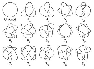

Links: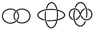

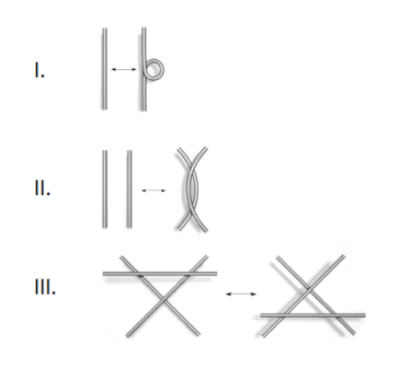
Reidemeister Moves

The Reidemeister moves are the three possible manipulations of knots that are used to find out if two diagrams represent equivalent knots. None of them physically change the knot, because they don’t make any cuts or make the knot intersect itself, so if the two diagrams are equivalent, they are related through a sequence of these three moves:

The Bracket Polynomial

There are many cases where it is difficult to deduce properties of a knot based solely on its diagram, which is why mathematicians have come up with algebraic ways to express knots, one of which is the bracket polynomial. This turns the knot into a polynomial expression by undoing each crossing one at a time, either horizontally or vertically, and describing the operation symbolically.

There are three relations bracket polynomials use when translating a knot into a polynomial:

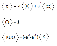
Here is a bracket polynomial worked out. It’s one of the more simple ones because the knot in question only has three crossings and is an unknot.

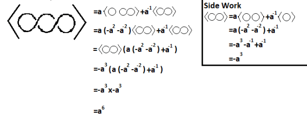
Bracket polynomials are invariant under Reidemeister moves 2 and 3, but not 1, meaning if you apply moves 2 or 3 to the knot, the resulting polynomial will remain the same, but when applying move 1, the resulting polynomial will change. Knowing a knot’s bracket polynomial is necessary to solve for its Kauffman polynomial.

 

Writhe Numbers

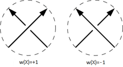
The writhe number of a knot is a numerical representation of its crossings. A crossing is equal to +1 if it’s positive, or crossing on top from left to right, and is equal to -1 if it’s negative, or crossing on top from right to left. Here’s the rule in symbols:

 

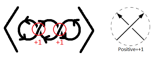
This unknot would have a writhe number of 2 because it has two positive crossings. In many cases, you need to orient the knot differently in order to see one of the two patterns above in a crossing, which is seen in the right crossing on the unknot below.

 

Writhe numbers, like bracket polynomials, are invariant under Reidemeister moves 2 and 3, but not 1. Knowing a knot’s writhe number is also necessary to solve for its Kauffman polynomial.

 

The Kauffman Polynomial

Another way of identifying knots algebraically is through their Kauffman polynomial. It requires both the knot’s bracket polynomial and writhe number in order to calculate it, but unlike the other two, the Kauffman polynomial is invariant under all of the Reidemeister moves. Here is its formula:

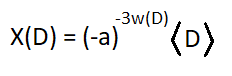
In the formula, D is the knot, w(D) is the writhe number,〈D〉is the bracket polynomial, X(D) is the Kauffman polynomial, and a is the variable. For the unknot we’ve been working with, <D> = a^6 and w(D) = 2. Here’s what we get when we plug them into the equation:

The end result is 1, which is to be expected because the knot shown is equivalent to the unknot, who’s writhe number is 0 and bracket polynomial is 1. As mentioned, the Kauffman polynomial is invariant under all of the Reidemeister moves, which means that all unknot equivalences will have a Kauffman polynomial of 1. This example was very simple because it was an unknot, but all knots that aren’t unknots will have a Kauffman polynomial dependent on variables.

We can use the Kauffman polynomial as proof for why the left handed trefoil and the right handed trefoil aren’t equivalent to each other:

If they were equivalent, their Kauffman polynomials would be the same, but because they’re not the same, we know that they are two completely different knots, despite them being mirror images of each other.