By: Michelle Chen, Cameron Farrar, Laura O’Sullivan, and Cat Bassett

Introduction

Everything we do in life has a chance. That chance may come from picking the right card, picking a certain marble out of a bag or maybe deciding to give the first person who walks through a random door $100. Essentially,each chance has a certain trade-off of benefits. Often times we think about the chances as something will happen over the chance of something else taking place as we weigh possible outcomes. This is called risk analysis. One of the ways we can determine risk is we can use Monte Carlo simulations to replicate real life situations a large number of times in order to observe the long-term patterns without having the complications (cost, labor, materials, etc.) of manual repetition.

Estimation of Pi

3.14159265358979323846264338327950288419716939937510582097494459230781640…

Pi. It’s a monster of a number that endless mathematicians have been attempting to conquer for centuries. Pi (π) is  a ratios of  a circle’s circumference to its diameter. However, because of its irrationality the number is extremely difficult to find.

However, we were able to use a simulation to come somewhere close.

What we did was we imagined that there was a circle of a radius of one inscribed in a square so that the square’s lines were tangent to the circle at four points as can be seen below.

Using prior knowledge, we know that the probability of “hitting” the circle would be (area of the circle or πr^2)/(area of the square or (2r)^2) which all simplifies to π/4. So, we know that the probability of hitting the circular area is π/4. Keep this in mind for later.

Then, using the middle of the circle and of the square as the origin, we generated random X and Y values between -1 and 1. Using the distance formula (X^2+Y^2=Distance^2) and the fact that all points on a circle are the same distance away from the origin, we determined whether or not certain points “hit” the circle based on how far away they were from the origin. If they were less than or equal to 1 (radius and shared distance by all points) away from the center, then the point hit the circle. If not, they were outside. Of course, more points meant more accuracy because patterns appear with more clarity in the long run.

Then, we found the proportion of points that hit the circle to the total number of points. This proportion should have equaled or should have been close to π/4 as we determined earlier. So, in order to find π, we multiplied the proportion we found by 4 in order to get an estimate of pi. Repeating this process several times with more points, we finally came up with the following table.

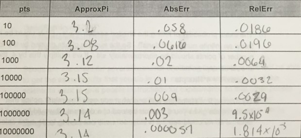
AbsErr of Pi: |ApproxPi-Pi|
RelErr of Pi: (AbsErr of Pi)/Pi

As you can see, more points lead to more accuracy. Though there’s error in all of the approximations, it progressively gets smaller which is sufficient for an approximation of pi.

It was pretty cool to make the code and to watch the accuracy improve throughout our trials. We ended up with a number very close to the π we’re familiar with which is awesome. One of our group members had previously only heard of one other method to estimate π so she thought it was cool that someone else had come up with this one.

1D Infection

In this problem we were told that a disease was spreading to 6 patients who were all in bed in a row. It said that the patient in the middle in the beginning has the disease. The way the disease spreads is that both people next to someone who is infected will get it, however a patient cannot have it for more than two days. After a patient has contracted and gotten over the illness, the patient can no longer get the disease again.

For our simulation, ,we had to keep the nature of the illness in mind (how long the illness lasted, the probability of getting the illness, how it spread, and how to account for those who became immune). We defined multiple variables such as probability (p) and length of illness (k) to help shape our simulation.

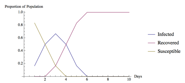
We see that by day six (when day one is defined as the day the first person gets the infection) all of the patients have had and become immune to the disease.

Visual 1

Black: Infected
White: Susceptible
Gray: Recovered

We are also able to observe the patients’ different states graphically as is displayed below.

Visual 2

2D Infection

This problem is very similar to the previous one with the exception that, instead of only simulating a single row of beds we are now observing multiple rows (and subsequently columns). So, we had to change the code in order to account for this change in dimensions.

Breaking down the problem, we realized that the disease would spread “upward” and “downward” in a sense as well as the horizontal motion from before. So, we needed a third variable to account for this type of motion.

It took us a bit longer to do this one too, because with the others we were shown how to, but with this one we had to take the 1D model and add in the new variable on our own, using the knowledge we gained from the previous problems. We also had to make sure that patient zero was still in the middle to get the pattern of movement we were hoping for.

Visual 1

---

Authors

Michelle: A rising senior by the time this is published, Michelle enjoys math and liked learning how to use Mathematica. She believe that her Girls Talk Math experience was amazing and would love to come back if she were able. In her free time, she enjoys watching dramas, reading books, and playing tennis. (In the podcast she’s the one with the puns you’re welcome).
Cameron: She is 16 years old and is a rising junior. Cameron enjoyed her Girls Talk Math experience more than she thought she would. She especially enjoyed the estimation of pi problem. In fact, being in the scientific computing group has encouraged her to learn coding on her own using Code Academy. In her free time, she enjoys playing basketball, studying absolutely anything and being involved in global health. She also likes the fact that Starbucks lets you use their wi-fi and bask in their air conditioning, making the store a great place to practice coding and meet with friends on a hot summer day.
Laura: At the time of this being published, she is a rising sophomore, she plays viola in her school orchestra and is a year ahead in math (starting Math 3 Honors). She feels that the Girls Talk Math Camp was a great opportunity that she was happy to be a part of. In her free time she enjoys watching a variety of T.V. shows and YouTube channels, reading/writing, and listening/playing music and is horrible at sports.
Cat: 17 years old and a rising senior, Cat (caitlyn) signed up for girls talk to help her with the upcoming AP calculus class she will be starting in the fall. She loved working and meeting all the girls from different parts of NC. In her free time she enjoys working with her high school marching band (she is the hopeful upcoming drum major). She also enjoys playing tennis, soccer, softball and swimming.

Check out our podcast on Grace Hopper at https://soundcloud.com/girls_talk_math/grace-hopper!