

By Tara Collins, Michelle Escobar, Kayla Rollins, and Logan White
When you hear the phrase computational dynamics, what comes to mind?

The struggle of programming can be all too real.
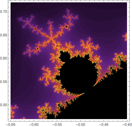
One of the many “bulbs” of the Mandelbrot Set.

What is computational dynamics?
A dynamic system, according to Wikipedia, is “a system in which a function describes the time dependence of a point in a geometrical space”.
In other words, it’s a mathematical way of showing how things change over time.
For example, a simple dynamic system could be a house. Imagine that this house only has one entrance and one exit. If you knew that two people entered the house every hour, but only one person exited it, you could write a function to show the behavior of the system– making it easy for you to know how many people are in the house at any given time!
No. of people in the house = (2 • hours passed) – 1

A graph of the function f(x) = 2x – 1.
This graph demonstrates the function we just described above– and it also illustrates where the computational component of dynamics comes into play.
Complex dynamic systems like the first one you saw are best described by computer-generated graphs, hence the “computational” portion of the phrase “computational dynamics”!
Functions, Iteration, and Orbits
Get your brain ready– this is where we’re going to cover all the important math concepts and lingo.
Iteration
Imagine the function f(x) = x². If we evaluated this function for the number 2, it would look like this:
f(2) = 2²
2² = 4
To iterate this function, we would take the value of f(2), which is 4, and plug it back into the same function:
f(4) = 4²
4² = 16
This process repeats infinitely.
2 is called our initial value and is denoted as x0. The values produced by an iteration are called the orbit of the initial value. So the orbit of f(x), x0 = 2, would look like this:
f(2) = 4
f(4) = 16
f(16) = 256
f(256) = 65, 536
….
And on and on. x0 = 2 gives us an infinitely increasing orbit, but what if our initial value were 1?
f(1) = 1
f(1) = 1
f(1) = 1
….
Interesting, right? The orbit doesn’t increase or decrease– in fact, it doesn’t change at all.
Orbits that continually increase or decrease are said to diverge, while orbits that repeat a pattern — like the one above — are said to be bounded.
Orbital Periods
When we have an orbit that repeats a certain pattern instead of zooming off to infinity, we say that it is periodic.
We define the period by how many values are in the repeated pattern.
So our example above — f(1) — has a period of 1, because it only repeats one value.
Let’s take the function f(x) = x² – 1 and iterate it for x0 = 0.
Programmer’s note: we can do this in Mathematica by using the command NestList. The values in the brackets represent NestList[ function name, initial value, number of iterations], where function name is the “name” of the function we’ve defined above, which is x² – 1 in this case. The output (in the curly brackets below) is the orbit of the initial value (0 in this example).
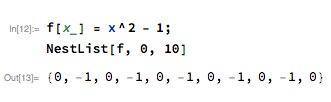
What do you think the period of this orbit is?
If you answered 2, then congratulations! You’re absolutely right.
(by the way, the period is 2 because the orbit cycles through 2 values — 0 and -1.)
Fixed Points
This concept can actually be described by a simple definition:
A point x0 is a fixed point for a function f(x) if f(x0) = x0.
Let’s break that down with an example.
For the function f(x) = x², two fixed points are 1 and 0. Why?
When we evaluate f(1), we get 1² = 1. The same thing occurs for 0 — 0² = 0.
Got it? Now we’re going to complicate things a little bit. There are two types of fixed points — attractive and repulsive.
An attractive fixed point is exactly what it sounds like — when you iterate a value near it, the orbit gets closer and closer to the actual value of the fixed point.

For the function f(x) = x², 0 is an attractive fixed point — when you take a value near 0, like 0.01, and iterate it, it draws closer to 0 itself.
As you might have guessed, a repulsive fixed point is the exact opposite — when you iterate a value near it, the orbit gets farther and farther away from the actual value of the fixed point.

For the function f(x) = x², 1 is an repulsive fixed point — when you take a value near 1, like 0.99, and iterate it, it is “repelled” and instead gets closer to 0.
And that’s it! Those are all of the basic concepts and terms you need to understand the coolest parts of computational dynamics.
The Mandelbrot Set
According to Google, the Mandelbrot set is “a particular set of complex numbers that has a highly convoluted fractal boundary when plotted.”
What?
Forget that definition. THIS is the Mandelbrot set:

Or, it’s a graphical representation of the Mandelbrot set, which is really just a series of mathematical expressions that meet these guidelines:
- They are functions of the form f(z) = z² + c,
- The initial value of z is always 0,
- Iterations of c have bounded periods.
If the orbit of c diverges, it’s not in the set!
And that’s really the fundamental concept of the Mandelbrot set. The mathematics behind it involves a lot of other calculations and concepts — like complex and imaginary numbers, derivatives, and cobweb plots — but it doesn’t take all of that to enjoy the visual and mathematical aspects of the Mandelbrot set.
Anyone can appreciate the number-based beauty that surrounds us — all it takes is a little bit of algebra and an eye for the exquisite.
Check out our podcast about mathematician Maryam Mirzakhani!
About the Authors:
Logan is a rising homeschooled senior who is thrilled and intrigued about all of the math and art in the world around her. Her favorite part of Girls Talk Math was not getting killed by Mathematica but instead conquering it! She also enjoyed learning an insane amount of math from her teachers and peers. Logan also has a night job as a Fictional Entity Analyst and Superhero Psychologist Extraordinaire.
Michelle is a rising freshman at Cardinal Gibbons who loves math, music and art. Her favorite part of Girls Talk Math was finally understanding the Mandelbrot Set and how to use Mathematica, as well as learning a bunch of different types of math and their applications!
Tara is a couch potato that loves chips. (She is actually a rising sophomore at Jordan who loves math, art and history.) My favorite part about Girls Talk Math is the potato chips!! And I guess the other campers.
 <–THIS IS TARA
Kayla is a rising freshman at J.D. Clements Early College at North Carolina Central University. She enjoys reading, writing, and playing sports. Kayla’s favorite part of Girls Talk Math was researching and doing a podcast on Maryam Mirzakhani. She also liked learning how to do and understand the Mandelbrot set plot.
